min read

Google Maps helps users find locations, plan optimal routes, and navigate with real-time traffic awareness.

Google Map

Written by

Staff Eng at Meta

Published on

April 12, 2025

Overview

1. An introductory note on shortest path algorithms —

In a system design interview for Google Map, the focus isn't on explaining algorithms like Dijkstra's, A*, or Bellman-Ford. While knowing these algorithms is valuable, the real challenge is how to apply shortest path algorithms efficiently to an enormous road network with:

Billions of road segments (edges)
Millions of intersections (vertices)
Real-time traffic conditions
Sub-second response requirements

The key is to discuss system-level optimizations and techniques that make these algorithms practical at scale.

2. Unique challenges with Google Map

Challenge with Design Yelp: Efficient proximity search — finding businesses based on location
Challenge with Design Uber: Handling massive scale real-time location updates from drivers

Design Google Map faces its own unique technical challenges:

Computing optimal routes with low latency on an extremely large road network graph
Calculating accurate ETAs by combining static graph data with real-time traffic conditions

Functional Requirements

(Location Search) Users can search for locations and receive corresponding physical addresses.
(Route Planning) Users can request and receive optimal routes between two locations.
(Navigation) Users can obtain turn-by-turn navigation instruction for their selected route.

Non-Functional Requirements

(Low Latency) The system should recommend routes and calculate ETAs with a low latency (p99 < 3seconds).
(Accuracy) The routes and ETAs must be accurate. Specifically:
- Routes should be "traversable" (no invalid road segments or turns).
- ETAs should be within ±10% of actual travel time for 90% of trips.
(High Availability) The system should maintain 99.99% uptime.
(Scalability) The system should scale horizontally to support X active users or Y requests per second (TBD), with the ability to handle peak (3 times more).

API Design

1. Location Search

GET /v1/geocode
{
    address: string,         // raw address (when user types an address)
    location: {              // optional, when user shares their current location
        lat: float,
        lng: float
    }
}
--> returns AddressInfo {
    formatted_address: string,
    place_id: string          // unique identifier for this location
    ...
}

2. Route Planning

GET /v1/routes?origin={some_address}&destination={some_address}

--> returns RouteInfo[] {
    duration: int, // estimated time in seconds
    distance: int, // in meters
    segments: RouteSegment[], // high-level route segments
    eta: string, // estimated arrival time
}

3. Navigation

GET /v1/directions/{route_id}

--> returns NavigationInfo {
    steps: DirectionStep[]   // detailed turn-by-turn instructions
    current_step: int,
    remaining_distance: int,
    remaining_time: int,
    next_maneuver: {
        instruction: string,  // e.g., "Turn right onto Market St"
        distance: int,        // distance until next maneuver
    },
}

High-level Design

We will skip the first functional requirement — "Users can search for locations and receive corresponding physical addresses" — since its solution is similar to what we covered in "Design Yelp". Instead, we'll focus on two more challenging requirements:

FR2: Route planning between two locations
FR3: Turn-by-turn navigation

These requirements present unique technical challenges specific to Google Maps.

Users can request and receive optimal routes between two locations.

Concept: Cell

Standard shortest path algorithms like Dijkstra's or A* cannot be directly applied to large-scale navigation systems due to the scale of modern road networks. These networks contain billions of vertices and edges, making direct path computation computationally intensive and memory-inefficient.

To solve this challenge, the road network graph is partitioned into smaller units called "cells" (also known as subgraphs, segments, or tiles in different contexts). Each cell represents a bounded geographical area containing a manageable portion of the road network that can be processed efficiently in memory. Within these cells, standard shortest path algorithms can effectively compute optimal routes between vertices. Each cell is defined by four coordinates (NW, NE, SW, SE) that determine its geographical boundaries, allowing us to model and store cells efficiently in a database.

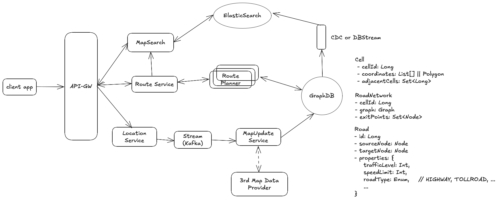
Data Model / Storage Schema

Cell - cellId: Long // Unique identifier for the cell - coordinates: List[] || Polygon // Geographic boundaries of the cell - adjacentCells: Set<Long> // IDs of neighboring cells

RoadNetwork - cellId: Long // Reference to containing cell - graph: Graph // Detailed road network within cell - exitPoints: Set<Node> // Border crossing points with adjacent cells Road - id: Long - sourceNode: Node // A road has two ends (start point, end point) - targetNode: Node - properties: { // Road attributes trafficLevel: Int, speedLimit: Int, roadType: Enum, // HIGHWAY, TOLLROAD, ... ... }

‍

Finding the shortest between two GEO points on a graph.

When a user requests navigation from point A to point B, the routing process follows a hierarchical approach operating at these two distinct levels:

Level 1: Cell Graph
- Nodes represent geographic cells
- Edges represent connections between adjacent cells
- Used for high-level path planning
Level 2: Road Graph
- Detailed road network within each cell
- Contains actual roads and intersections
- Used for precise route calculation

With two levels, we do two levels planning:

Cell-Level Path Planning First.
- Identifying the source cell containing point A
- Identifying the destination cell containing point B
- Computing the optimal sequence of cells to traverse using the shortest path algorithm
Detailed Route Calculation. Once the cell sequence is determined, the system computes the detailed route by:
1. Point-to-Road Mapping
  - Projects source point A onto its nearest road segment within the source cell
  - Projects destination point B onto its nearest road segment within the destination cell
  - Each projection creates a temporary routing point on the actual road network.
  - (Notes on projection) Real-world locations often aren't exactly on roads. So we need to connect arbitrary points to a node on our graph for routing. Projection is a process to find the closest road segment (”Node”) to a user specified point and then route planning will use that road segment as the starting point.
2. Within-Cell Routing
  - For each cell in the sequence, computes optimal paths between:
    - Source point to cell exit points (in first cell)
    - Entry points to exit points (in intermediate cells)
    - Entry points to destination (in last cell)
  - Uses standard shortest path algorithms on the detailed road network within each cell
3. Path integration (combine the results of within-cell routing + cell-level planning)
  - Connects all sub-paths between cells.
  - Produces final continuous route from A to B

#Optimization techniques# The above route planning process could work to find a path between two points. But it is not efficient because

Cell graph could still be very large (on a globe scale);
Each cell's four exit points create redundant calculation on finding the closest exit point.

Here are the techniques to improve:

1. Distance-Based Search Reduction
- Calculate straight-line (Euclidean) distance between cells
- Prune search paths that exceed known better routes
Example: If we find a 12km route, we can skip exploring paths that:
- Exceed 12km from source
- Have a straight-line distance to destination beyond the remaining allowance
2. Exit Point Distance Caching
- Pre-compute distances to exit points
- Cache results in the road table
- Eliminate redundant calculations during path finding

We had briefly talked about two techniques on making route planning fast:

Using distance to reduce the search space;
Pre-computing the distance to exist point and adding them to cache;

We will explore more in deep dive section (i.e: split graph DB into multiple shard, have [Route Planner] handle one/multiple cell(s) and then do "within cell planning" in parallel)

Get an optimal path considering real-world traffics conditions.

So far we have just discussed how to find a theoretically shortest path based on static road networks (or all roads have the same weights). In a real-world scenario, the shortest path may not be the quickest or the optimal path. We have to consider road or traffic condition. Those signals (road condition, traffic condition) can be collected from users/drivers.

(High-level Idea) When drivers use the app, their devices periodically report telemetry data including current location, speed. This data provides insights to actual road conditions. Then our system processes this raw telemetry data to derive current traffics conditions for each road segment.

Traffic conditions are quantified by comparing real-time vehicle speeds against the road's design speed. For a road segment with a design speed of 60 kilometers per hour, traffic levels are categorized based on the 90th percentile of observed vehicle speeds. For example,

(No traffic) Over 90% of vehicles travel at a speed of 60 KM/H or higher.
(Light traffic) Over 90% of vehicles travel at speed between 48 ~ 60 KM/H;
(Medium traffic) Over 90% of vehicles travel at a speed between 30 ~ 48KM/H;
(Heavy traffic) Over 90% of vehicles travel at a speed less than 30 KM/H.

We can assign weight multipliers (i.e: 1.0, 1.3, 1.5, 1.8) to road segments based on these traffic levels. These weights directly impact route selection and travel time estimation during path calculation. Less congested routes may be favored even they may be physically longer.

Our design is purely based on “the speed signal” reported from drivers. In reality, GoogleMap might use a much sophisticated algorithm which considers many more factors such as average vehicle speed, traffic density (# cars on a road), and historical patterns (the average speed for 7 - 9 AM based on last 30-days data)..
‍‍

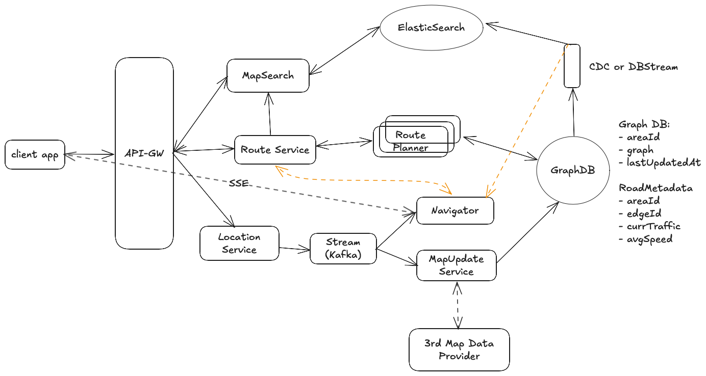
Designed workflow

Here is our final workflow with everything discussed so far

User sends a route planning request with source and destination address. GET /v1/routes?origin={some_address}&destination={some_address}
API-GW routes this request to [Route Service]. [Route Service]
- queries [MapSearch] service to identify which geographic cells contain the source and destination location;
- computes the optimal sequence of cells to traverse;
- (for each cell in the sequence) sends request to [Route Planner] to find the path within a cell;
[Route Planner] queries RoadNetwork and Road table from our graph database and run the shortest path algorithm (A* search) to calculate the path (within a cell) considering traffic conditions.
[Route service] aggregates and produces the final complete route between source and destination using all results returned from [Route Planner]. This final route is then returned to the user, complete with turn-by-turn directions and estimated travel time.

Users can obtain turn-by-turn navigation instruction for their selected route.

In FR2, [Route Service] returns turn-by-turn directions and estimated travel time. Once user accepts the recommend route (directions), navigation process will start.
(On the client side) Client App renders/displays the turn-by-turn directions and starts tracking user’s current location and continuously report user’s current location.
Handle route deviation
- If client app detects user’s current location is no longer on the recommended path, it sends a request (GET /v1/routes) with current location and original destination.
- [Route Service] calculates and returns new route.
- Client App renders and displays new route in the app.

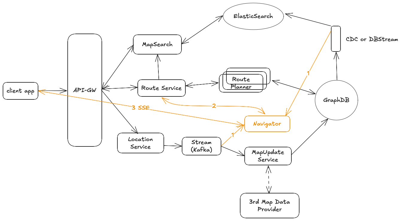
Dynamic Route Monitoring and Suggestion (refer to the yellow line in diagram)

Modern navigation systems like Google Maps can dynamically recommend better routes as traffic conditions change. Instead of only responding when users deviate from their route, the system actively monitors upcoming traffic conditions and suggests faster alternatives before users encounter delays. For example, if there's unexpected congestion 5 miles ahead that would add 15 minutes to your trip, the system can notify you about an alternate route that avoids that traffic, even though you haven't reached the congestion yet.

We will add an additional backend service [Navigator Service] , which consumes messages from two data streams: [1] database updates and [2] user’s current location.
When a user begins navigation, the [Navigator Service] tracks all road segments in their chosen route. It monitors both traffic data streams from the database (using driver telemetry data) and location updates from the Kafka stream. If significant changes occur - such as a traffic level shifting from light to heavy, the [Navigator Service] evaluates the impact on the total journey time.
When these changes would affect the estimated arrival time by 5% or more (either slower or faster), the [Navigator Service] initiates a re-route process. It requests a new route calculation from the [Route Service] using the user's current location and original destination. If a better route is found, this information, along with current traffic conditions, is immediately pushed to the user's device through Server-Sent Events (SSE).

Deep Dive

The system should recommend routes and calculate ETA within 3 seconds for 95% requests;

Beyond our previously discussed techniques (distance-based search space reduction and exit point pre-computation), we can implement additional optimizations:

Parallel Route Computation
- Partition road network graph across multiple database shards
- Each shard contains a subset of cells
- Route Planner instances handle specific cell groups
- Enables parallel computation of within-cell paths
- Results are aggregated by Route Service
Caching Strategy
- Cache frequently requested routes during peak hours
- Maintain cell-level traffic summaries
- Store pre-computed distances between major intersections

The system should be highly available and can tolerance component failures.

Handle Kafka stream failures
- Configure each topic with replication factor of 3, meaning every message is stored on three different brokers. So we have tolerance on broker failure.
- Enable message persistence (retention period of 24 hours). Say if Navigator Service misses messages (or goes down for 10 seconds), it can replay/request messages from last successful offset.
Handle individual component failures
- Setup monitoring to monitor service health (i.e: resource utilization, throughput, processing latency etc).
- Automatically failover to secondary instance once primary server is down or not responding;
- Employ a rate limiter in front of all services to ensure service is not overloaded with huge number of requests.

The routes and ETA produced by the system should be highly accurate .

Map Data Freshness
- Sync with 3rd map data provider frequently to keep our map fresh/up-to-date;
- Do emergency updates on major changes (road closures, new constructions etc);
Adaptive Location Update based on context
- High-density areas: Updates every 3-5 seconds
- Highway driving: Updates every 10-15 seconds based on speed
- Complex intersections: Increased frequency to 1-2 seconds
- Approaching decision points: More frequent updates
Dynamic Route Monitoring and Suggestion (already discussed in HLD).
(say if you have ML expertise) Apply ML algorithm on route planning and ETA calculation by training historical data.

The system should be able to scale to support X QPSs

Horizontally scale individual service components (i.e: [Route Service], [Route Planner])
Regionalization.
- Deploy the system into more regions (US-West, US-East, EU, Asia).
- Have local deployed system to serve local users.

‍

Coach + Mock

Practice with a Senior+ engineer who just get an offer from your dream (FANNG) companies.

Schedule Now

Content: